import numpy as np
import matplotlib.pyplot as plt
import scipy as sp
import pandas as pd
import datetime as dt

# Set random seed for reproducibility
np.random.seed(42)

# Set plotting style
plt.style.use("ggplot")
plt.rcParams['figure.figsize'] = [10, 6]  # Default figure size
TRADING_DAYS = 251def generate_stock_data(
num_days: int = 251, # Default to one trading year
initial_price: float = 100.0,
annual_return: float = 0.1, # 10% annual return
annual_volatility: float = 0.2, # 20% annual volatility
) -> pd.DataFrame:
"""
Generate synthetic stock price data using geometric Brownian motion.
Parameters:
- num_days: Number of trading days
- initial_price: Starting price of the stock
- annual_return: Expected annual return (mu)
- annual_volatility: Annual volatility (sigma)
"""
# Daily parameters
daily_return = annual_return / num_days
daily_volatility = annual_volatility / np.sqrt(num_days)
# Generate random returns
np.random.seed(42) # For reproducibility
daily_returns = np.random.normal(
loc=daily_return,
scale=daily_volatility,
size=num_days
)
# Calculate cumulative returns
cumulative_returns = np.exp(np.cumsum(daily_returns))
# Generate price series
prices = initial_price * cumulative_returns
# Create dates
dates = pd.date_range(
start=dt.datetime.now() - dt.timedelta(days=num_days),
periods=num_days,
freq='B' # Business days
)
# Create DataFrame
return pd.DataFrame(
{'Close': np.insert(prices, 0, initial_price)},
index=pd.date_range(
start=dates[0] - dt.timedelta(days=1),
periods=len(prices) + 1,
freq='B'
)
)One of the fundamental principles in finance, often attributed to Paul Wilmott, states that “the level of price doesn’t matter, only returns matter.” This is a fascinating observation because while we model asset prices, they rarely appear directly in our equations. Instead, our focus is consistently on returns.
Simple vs Log Returns
Having previously explored the advantages of logarithmic returns in our time series analysis, let’s revisit this important concept before delving deeper into quantitative finance topics. Understanding the differences between simple and logarithmic returns is crucial for financial modeling.
Simple Multi-Period Return
For compound returns, we begin with the discrete compounding formula: \[ S_T=S_0\left[1+\frac{r}{T}\right]^{Tt} \] where: - \(S_0\) is the initial investment - \(t\) is the total duration (usually in years) - \(r\) is the annual return - \(T\) is the number of compound periods (days, weeks, or seasons)
When we take the compound period to be infinitesimally small (continuous compounding), we obtain: \[ \lim _{T \rightarrow \infty} S_T=S_0 e^{rt} \] This continuous compounding formula is fundamental to many financial models, particularly in derivatives pricing.
Note: When modeling over a one-year period, we often omit \(t\) from the equations since \(t=1\).
The following plot demonstrates how discrete compounding converges to continuous compounding as we increase the number of compound periods. This convergence is a key principle in understanding why continuous compounding models are often preferred in financial mathematics.
S_0 = 1000
r = 0.05
t = 1

S_T_continuous = S_0 * np.exp(r * t)

compound_periods = range(1, 101)
S_T_discrete = [S_0 * (1 + r / n) ** (n * t) for n in compound_periods]

fig, ax = plt.subplots(figsize=(9, 4))
ax.plot(
    compound_periods,
    S_T_discrete,
    label="Discrete",
    linestyle="--",
    marker="o",
    color="blue",
)
ax.axhline(y=S_T_continuous, color="r", linestyle="-", label="Continuous")
ax.set_xlabel("Number of Compounding Periods (n)")
ax.set_ylabel("Future Value (S_T)")
ax.legend()
plt.title("Continuous vs. Discrete Compounding")
plt.show()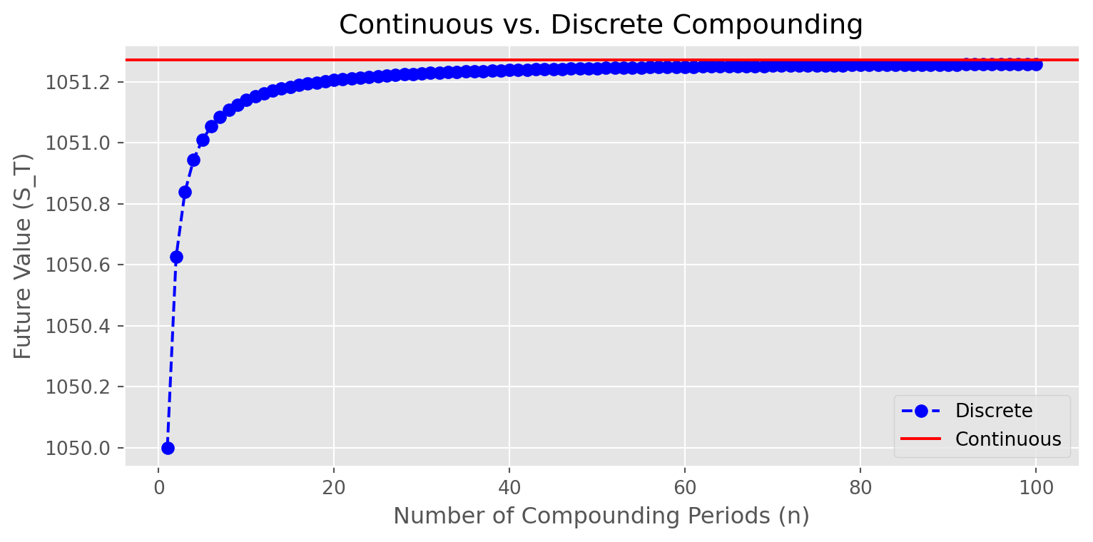
Simple Returns Simulation
To model real-world financial returns, we introduce a stochastic (random) component to the simple return at each period \(t\). This addition helps capture the inherent uncertainty and volatility in financial markets.
\[\begin{aligned} r_t= & \frac{S_t-S_{t-1}}{S_{t-1}} \\ & =\frac{r}{T}+\frac{\sigma}{\sqrt{T}} \varepsilon_t \quad \varepsilon_t \sim N(0,1)\end{aligned}\]
The \(\sqrt{T}\) term in the equation arises from a fundamental property of standard deviation: when summing independent random variables, their variances add linearly, but standard deviations scale with the square root of the number of periods. This is why we often see square roots in financial formulas involving time scaling of volatility.
def simple_return_simulation(
    s0: float = 100,
    r: float = 0.1,
    vol: float = 0.10,
    trading_days: int = TRADING_DAYS,
    paths: int = 100,
) -> None:
    """
    Simulate multiple price paths using simple returns with random components.

    Parameters:
    -----------
    s0 : float, default=100
        Initial price
    r : float, default=0.1
        Annual return (10% by default)
    vol : float, default=0.10
        Annual volatility (10% by default)
    trading_days : int, default=251
        Number of trading days to simulate
    paths : int, default=100
        Number of simulation paths to generate

    Returns:
    --------
    None
        Displays a plot showing all simulated paths and their final distribution
    """
    # Generate standard normal random numbers for all paths
    norm_draws = np.random.randn(paths, trading_days)

    # Calculate daily parameters
    daily_return = r / trading_days
    daily_vol = vol / np.sqrt(trading_days)

    # Generate daily gross returns (1 + simple return)
    gross_returns = 1 + daily_return + daily_vol * norm_draws

    # Add initial value (1.0) at the start of each path
    gross_returns = np.insert(gross_returns, 0, 1.0, axis=1)

    # Calculate cumulative returns through multiplication
    cumulative_returns = s0 * np.cumprod(gross_returns, axis=1)

    # Create the plot
    fig, ax = plt.subplots(figsize=(14, 7))

    # Plot all paths
    time_points = np.arange(trading_days + 1)
    for path in cumulative_returns:
        ax.plot(time_points, path, linewidth=0.7, alpha=0.6)

    # Customize main plot
    ax.set_title("Simple Return Simulation: Multiple Price Paths Over One Year",
                fontsize=20)
    ax.set_xlabel("Trading Days", fontsize=16)
    ax.set_ylabel("Price", fontsize=16)

    # Add histogram of final values
    ax_hist = ax.twinx()
    ax_hist.set_yticks([])
    ax_hist.hist(
        cumulative_returns[:, -1],  # Final values of all paths
        bins=50,
        orientation="horizontal",
        alpha=0.3,
        color="grey",
        density=True
    )
    ax_hist.set_ylabel("Distribution of Final Values", fontsize=16)

    # Add statistical summary
    final_values = cumulative_returns[:, -1]
    stats_text = (
        f"Final Value Statistics:\n"
        f"Mean: ${final_values.mean():.2f}\n"
        f"Std: ${final_values.std():.2f}\n"
        f"Min: ${final_values.min():.2f}\n"
        f"Max: ${final_values.max():.2f}"
    )
    ax.text(0.02, 0.98, stats_text,
            transform=ax.transAxes,
            verticalalignment='top',
            bbox=dict(boxstyle='round', facecolor='white', alpha=0.8))

    plt.tight_layout()
    plt.show()
# Generate synthetic stock data
data = generate_stock_data(
num_days=TRADING_DAYS,
initial_price=100.0,
annual_return=0.1, # 10% annual return
annual_volatility=0.2 # 20% annual volatility
)data| Close | |
|---|---|
| 2024-10-14 18:55:59.381683 | 100.000000 |
| 2024-10-15 18:55:59.381683 | 100.669116 |
| 2024-10-16 18:55:59.381683 | 100.533603 |
| 2024-10-17 18:55:59.381683 | 101.399360 |
| 2024-10-18 18:55:59.381683 | 103.408974 |
| ... | ... |
| 2025-09-24 18:55:59.381683 | 107.423413 |
| 2025-09-25 18:55:59.381683 | 106.583531 |
| 2025-09-26 18:55:59.381683 | 109.029045 |
| 2025-09-29 18:55:59.381683 | 109.631546 |
| 2025-09-30 18:55:59.381683 | 107.943324 |
252 rows × 1 columns
data["simple_return"] = data.pct_change()
data_mean = data["simple_return"].mean() * TRADING_DAYS
data_std = data["simple_return"].std() * np.sqrt(TRADING_DAYS)
# Example of using the generate_stock_data function
generate_stock_data(
num_days=TRADING_DAYS,
initial_price=100.0,
annual_return=0.1,
annual_volatility=0.2
)| Close | |
|---|---|
| 2024-10-14 18:55:59.421177 | 100.000000 |
| 2024-10-15 18:55:59.421177 | 100.669116 |
| 2024-10-16 18:55:59.421177 | 100.533603 |
| 2024-10-17 18:55:59.421177 | 101.399360 |
| 2024-10-18 18:55:59.421177 | 103.408974 |
| ... | ... |
| 2025-09-24 18:55:59.421177 | 107.423413 |
| 2025-09-25 18:55:59.421177 | 106.583531 |
| 2025-09-26 18:55:59.421177 | 109.029045 |
| 2025-09-29 18:55:59.421177 | 109.631546 |
| 2025-09-30 18:55:59.421177 | 107.943324 |
252 rows × 1 columns
simple_return_simulation(s0=100, r=data_mean, vol=data_std, trading_days=251, paths=500)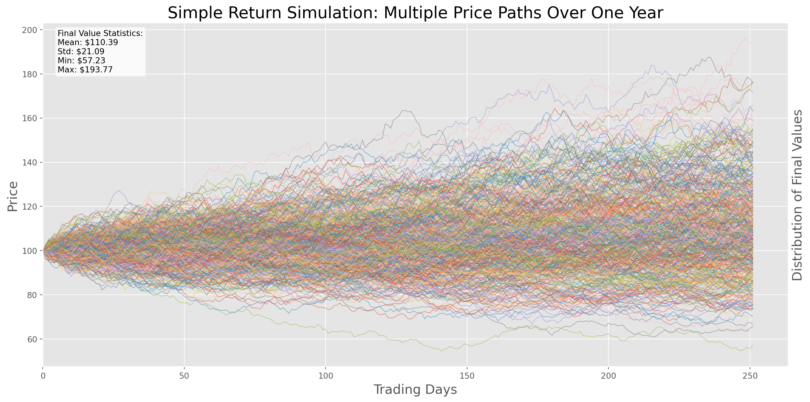
An important limitation of simple returns is their multiplicative nature: \[ \left(1+r_1\right)\left(1+r_2\right) \ldots \left(1+r_T\right)-1=\prod_{i=0}^T\left(1+r_i\right)-1 \]
This multiplicative property means that the product of simple returns does not follow a normal distribution, even when the individual returns are normally distributed. This non-normality can complicate statistical analysis and modeling.
Log Return
One of the key advantages of continuous compounding is its additive property in the exponential term. We can demonstrate this mathematically: \[ \begin{aligned} S_T & =S_0e^{\frac{r}{T}}e^{\frac{r}{T}} \ldots e^{\frac{r}{T}} \\ & =S_0 e^{\frac{r}{T}+\ldots+\frac{r}{T}} \\ & =S_0 e^r \end{aligned} \]
This property makes continuous compounding particularly useful for mathematical analysis and modeling.
Divide \(S_0\) on both side and take natural log, we obtain log return at period \(T\) \[ \log{\left(\frac{S_T}{S_0}\right)}=\log{e^r} = r_{_T}[T] \] The notation is consistent with what we had in time series session, \(r_{_T}[T]\) means \(T\) periods log return.
What’s more, we can decompose gross return into additive log returns \[ \begin{align} \log{\left(\frac{S_T}{S_{T-1}}\frac{S_{T-1}}{S_{T-2}}\ldots\frac{S_1}{S_0}\right)} &= \log{\left(\frac{S_T}{S_{T-1}}\right)} \log{\left(\frac{S_T}{S_{T-1}}\right)} \ldots\log{\left(\frac{S_T}{S_{T-1}}\right)}\\ r_{_T}[T]&= \underbrace{r_{_{T-1}} + r_{_{T-2}}+\ldots+r_{_0}}_{T \text{ periods}} \end{align} \] This is the additive feature of log return.
Note that \(r_{_T}[T]\neq r_{_T}\), the former one is an accumulative return the later is a single period return.
In contrast to simple returns, \(r_{_T}[T]\) follows a normal distribution, because it’s a linear combination of \(T\) normal distributions of \(r\).
Simulation of Log Return
Similarly, we add random components on to log return
\[ \ln \left(\frac{S_T}{S_0}\right)=r+\sigma \varepsilon_t, \quad \varepsilon_t \sim N(0,1) \]
So Which One to Use?
The choice between simple and logarithmic returns depends on your specific needs:
- For individual investors focused on basic portfolio management, either approach may be suitable as the differences are often minimal for short time periods and small returns.
- For institutional investors and quantitative researchers, this choice is fundamental and must be made early in the modeling process, as it affects everything from risk assessment to portfolio optimization.
The decision should be based on your specific use case, the mathematical properties you need to preserve, and the type of analysis you plan to perform.
The merit of simple return: simple returns are asset-additive.
The portfolio return can be added up together \[ R_p=\sum_{i=1}^k w_i R_i \] where \(R_p\) is portfolio return, \(w_i\) and \(R_i\) are weight and simple return of asset \(i\).
In contrast, log returns are time-additive, i.e. \[ r_{_T}[T]= r_{_{T-1}} + r_{_{T-2}}+\ldots+r_{_0} \]
In fact, log returns are not a linear function of asset weights. That is, a portfolio’s log return does not equal the weighted average of the log returns of the assets in the portfolio.
The log return of portfolio \(r_p\) mathematically will be \[ r_p=\log \left(\sum_{i=1}^N w_i e^{r_i}\right) \] where \(w_i\) and \(r_i\) are weight and log return of asset \(i\). Obviously this is no longer a linear function.
Comparison Experiment
Let’s generate synthetic data for two assets (Asset A and Asset B) and use weights \([0.6, 0.4]\) to calculate the portfolio return.
We’ll calculate the log return of each asset, but use the additive method for calculating the portfolio return. We’ll use this return to compare with the correct simple portfolio return, and we expect to see a discrepancy between them.
# Generate data for two assets
asset_a = generate_stock_data(
    num_days=TRADING_DAYS,
    initial_price=100.0,
    annual_return=0.1,
    annual_volatility=0.2
)

asset_b = generate_stock_data(
    num_days=TRADING_DAYS,
    initial_price=50.0,
    annual_return=0.05,
    annual_volatility=0.1
)

# Combine into a single DataFrame
data = pd.DataFrame({
    'Asset_A': asset_a['Close'],
    'Asset_B': asset_b['Close']
})

# Calculate returns
data_simple_return = data.pct_change(fill_method=None).dropna()  # Explicitly set fill_method
data_log_return = np.log(data).diff()  # More efficient way to calculate log returns

# Portfolio weights
weights = np.array([0.6, 0.4])

# Calculate annualized portfolio returns
simple_portfolio_return = np.sum(data_simple_return.mean() * weights) * TRADING_DAYS
mixed_portfolio_return = np.sum(data_log_return.mean() * weights) * TRADING_DAYS

print("Annualized Simple Portfolio Return: {:.2%}".format(simple_portfolio_return))
print("Annualized Log-based Portfolio Return: {:.2%}".format(mixed_portfolio_return))

# Also show the difference
print("\nDifference between methods: {:.2%}".format(
    simple_portfolio_return - mixed_portfolio_return
))
Annualized Simple Portfolio Return: 0.00%
Annualized Log-based Portfolio Return: 0.00%
Difference between methods: 0.00%So you have to be consistent about when to use which. In general for time series modeling, log return is your choice, when comes to portfolio optimization or management, simple return would be more accurate.
Standardized Return vs Normal Distribution
Standardized returns are a crucial tool in financial analysis for several reasons:
- They allow us to compare returns across different assets and time periods on an equal basis
- They help identify extreme market events by measuring how many standard deviations an observation deviates from the mean
- They facilitate the assessment of whether returns follow a normal distribution
In real markets, we often observe returns that are many standard deviations away from the mean (known as “fat tails”), which occur more frequently than a normal distribution would predict. This observation has important implications for risk management.
def standardized_return(simple_return):
    return (simple_return - simple_return.mean()) / np.std(simple_return, axis=0)
n = 300
norm_pdf = sp.stats.norm.pdf(np.linspace(-10, 10, n), loc=0, scale=1)
x_ticks = np.linspace(-10, 10, n)Compare with standard normal distribution.
fig, ax = plt.subplots(figsize=(14, 6), nrows=1, ncols=2)
ax[0].hist(
    standardized_return(data_simple_return)["Asset_A"], bins=100, density=True, label="Asset A"
)
ax[1].hist(
    standardized_return(data_simple_return)["Asset_B"], bins=100, density=True, label="Asset B"
)
ax[0].plot(x_ticks, norm_pdf, lw=3, label="Normal")
ax[1].plot(x_ticks, norm_pdf, lw=3, label="Normal")
ax[0].legend()
ax[1].legend()
ax[0].set_title("Asset A Returns vs Normal Distribution")
ax[1].set_title("Asset B Returns vs Normal Distribution")
plt.show()
/home/runner/.cache/pypoetry/virtualenvs/workspace-env-xqASYfE0-py3.12/lib/python3.12/site-packages/numpy/lib/histograms.py:885: RuntimeWarning:
invalid value encountered in divide
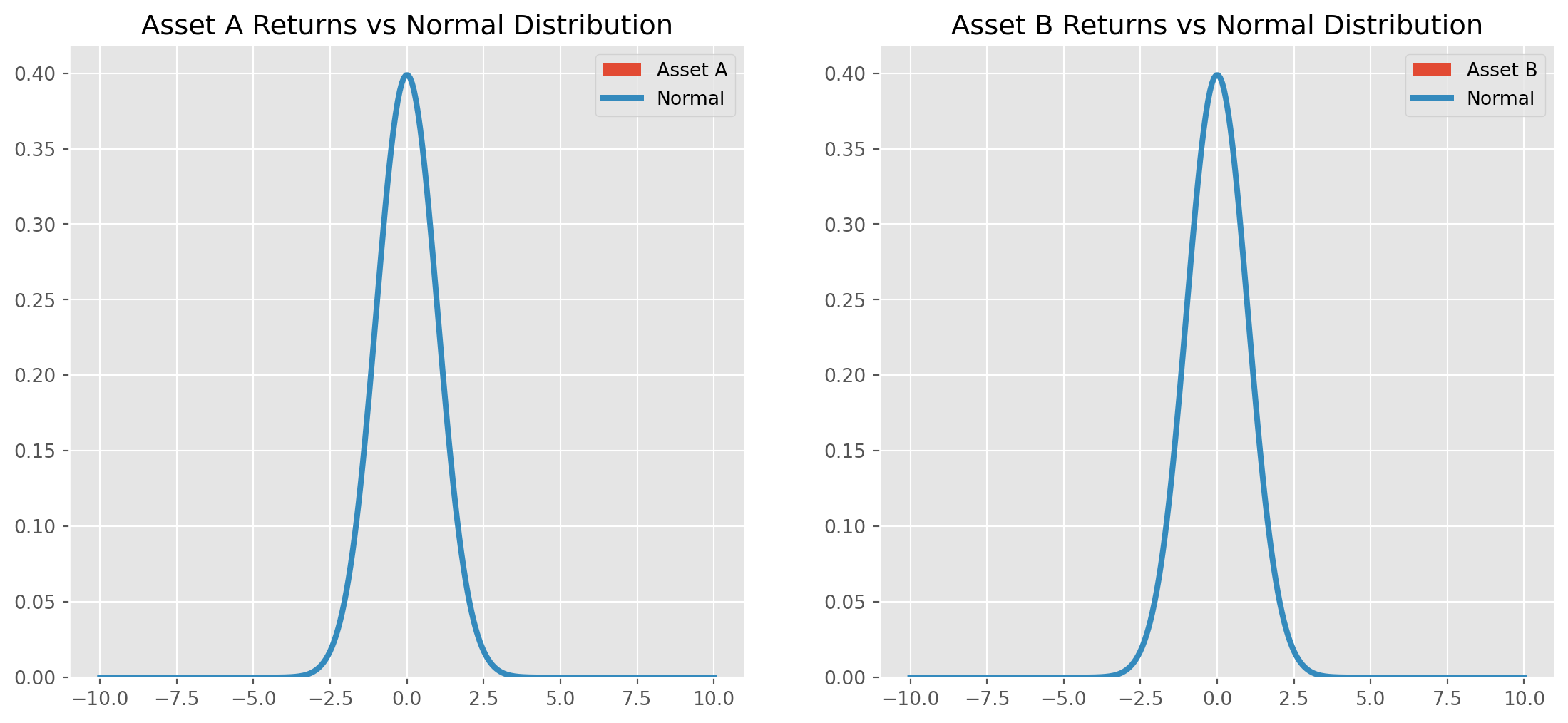
The return distribution is not Gaussian; however, why do we persist in using the normal distribution in practice? There are several reasons: the normal distribution has a closed-form function, is defined by just two parameters, and the central limit theorem assures its applicability and a finite standard deviation.
Conversely, as demonstrated by the histograms, the fat-tailed distribution may lack a closed-form probability density function (pdf), and most critically, its standard deviation can be infinitely large.
Therefore, insisting on using a fat-tailed model can sometimes make modeling impractical due to the possibility of an infinite standard deviation.
Despite the extremely low probability of fat tails, we still need to have a strategy for handling them.
Assets Return Modeling
We have explored two models previously: one discrete and the other continuous. \[ S_T=S_0\left[1+\frac{r}{T}\right]^{Tt},\qquad\lim _{T \rightarrow \infty} S_T=S_0 e^{rt} \] These notations are more commonly encountered in time series analysis.
In the realm of financial engineering, however, we typically express these models as follows: \[ S_M = S_0(1+\mu \delta t)^M, \qquad\lim _{\delta t \rightarrow 0} S_M=S_0 e^{\mu M \delta t} = S_0 e^{\mu t} \] Here, \(M=\frac{t}{\delta t}\) represents the number of intervals, and \(\mu\) denotes the annual return. For example, when modeling daily data in the United States, we use \(\delta t = 252\) which has been defined as a constant at the top of this notebook.
Now suppose you know annualized standard deviation of return \(\sigma\), the variance over \(M\) periods (can be days, months or years) will be \[ \sum_{i=1}^{M}\sigma^2 = M \sigma^2 = \frac{t}{\delta t}\sigma^2 \]
If we set \(t=1\), i.e. one year period (252 trading days), we obtain variance over \(1/\delta t\) periods, because variance is additive \[ \frac{1}{\delta t}\sigma^2 \]
Naturally, the standard deviation over \(1/\delta t\) periods should be the square root of it \[ \frac{\sigma}{\sqrt{\delta t}} \]
So if you know annualized \(\sigma = .30\), what’s the standard deviation over a day? \[ \frac{\sigma}{\sqrt{252}} = \frac{0.30}{\sqrt{252}} \]
In contrast, the time unit conversion of mean is straightforward, the mean over certain period of time \[ \mu \ \delta t \] where \(\mu\) is annualized return, e.g. \(\mu=0.08\), daily return is \[ 0.08 \times \frac{1}{252} \]
Now join what we have discussed together, we can write a model for asset returns \[ R_{t} = \frac{S_{t+1}-S_t}{S_t} = \mu \delta t+\varepsilon \sigma \sqrt{\delta t} \] where \(\varepsilon\) is a variable drawn from normal distribution (doesn’t have to be standard normal).
Actually this is a famous stochastic process model named generalized Wiener Process.
Assets Price Level Modeling
With a slight modification of previous model \[ S_{i+1}-S_i=\mu S_i \delta t+\varepsilon S_i \sigma\sqrt{\delta t}\quad\Rightarrow\quad S_{i+1}=(1+\mu \delta t) S_i+\varepsilon S_i \sigma\sqrt{\delta t} \]
Insights
Take a close look at the model \[
S_{i+1}-S_i=\mu S_i \delta t+\varepsilon S_i \sigma\sqrt{\delta t},\\
\text{ or}\\
S_{i+1}=(1+\mu \delta t)S_i+\varepsilon S_i \sigma\sqrt{\delta t}
\] This is exactly what I was doing in codes above [1 + r / trading_days + vol / (np.sqrt(trading_days))]! The only difference is that we were simulating cumulative returns rather than price.
On the left-hand side, \(\delta t\) appears twice, i.e. \(\delta t\) and \(\sqrt{\delta t}\).
From the plot, we understand that for \(0<\delta t < 1\), it follows that \(\delta t<\sqrt{\delta t}\). As \(\delta t\) approaches \(0\), the term \(\varepsilon S_i \sigma\sqrt{\delta t}\) becomes increasingly dominant. This indicates that our model focuses primarily on volatility over extremely short time periods.
In simpler terms, this means that in the short term, random fluctuations significantly outweigh the overall growth (or drift), as you can see from the plot below, the slop of the square root curve infinitely converges to \(1\) as the interval converges to \(0\).
x = np.linspace(0, 1.3)
y = np.sqrt(x)
fig, ax = plt.subplots(figsize=(7, 7))
ax.plot(x, y, label=r"$y = \sqrt{\delta t}$")
ax.plot(x, x, label=r"$y = \delta t$")
ax.scatter(1, 1, color="red", s=100)
ax.legend()
plt.show()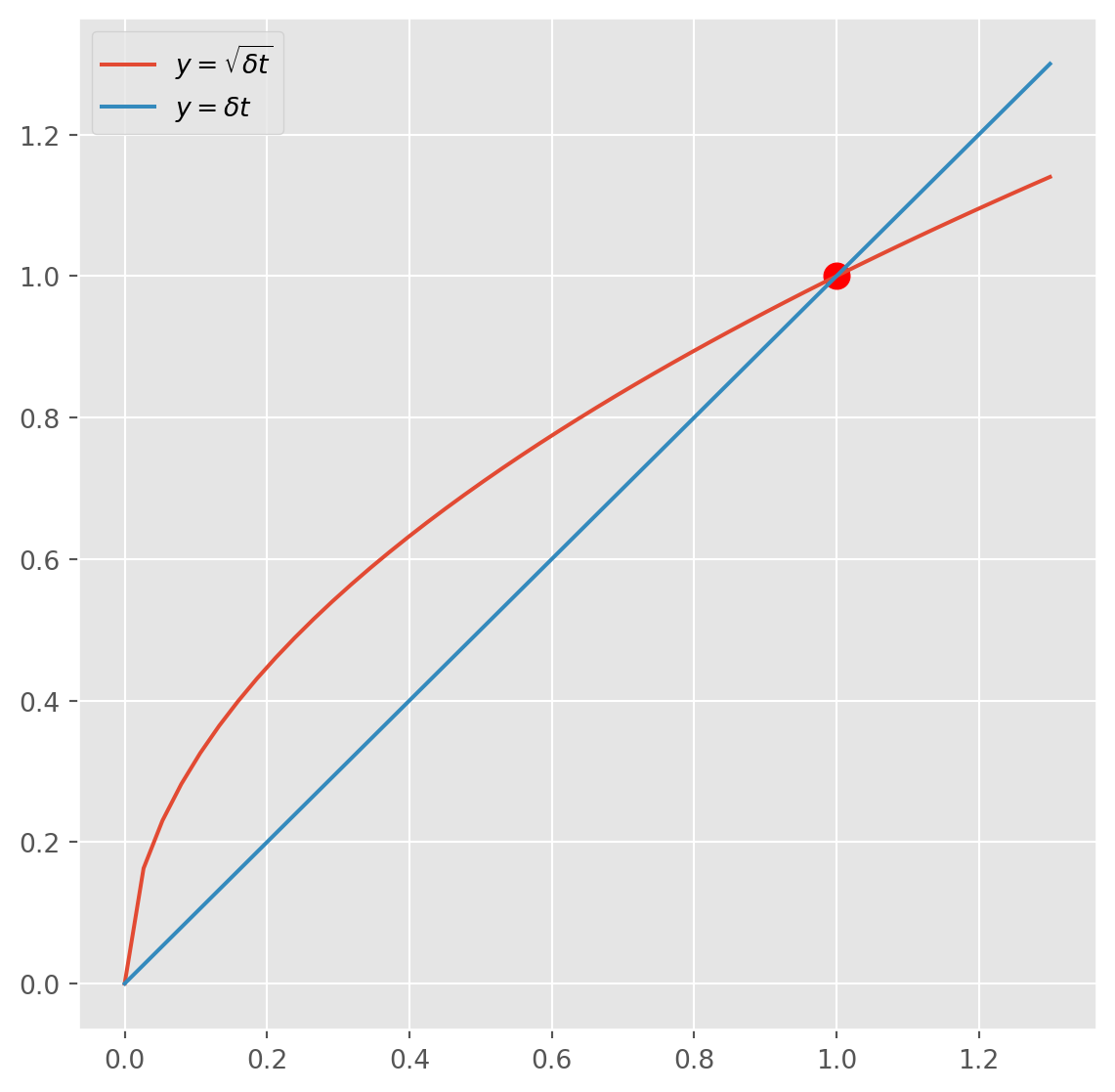
For the sake of mathematical convenience, many people will be using continuous version of this model, i.e. \[ d S=\mu S d t+\sigma S d X \] where \(E[d X]=0\) and \(E\left[d X^2\right]=d t\). A full derivation will be carefully discussed in later chapters, because this is the foundation of all other quantitative financial models.